Exploring Stock Data

I have recently been intrested in modeling stock volatility. In order to make the process easier, I wanted a way to quickly download stock data in R, and after some quick searching on the web, I stumbled across the tidyquant package which is able to download stock data from Yahoo Finance, and then conveniently store the data as a tibble object.

I decided to download the data for the ten largest weighted Dow Jones Industrial Average stocks.

library(tidyquant)
stockDF <- tq_get(c("AAPL", "UNH", "HD", "GS", "MCD", "V", "MSFT", "MMM", "JNJ", "BA"))
str(stockDF)

## tibble [26,390 × 8] (S3: tbl_df/tbl/data.frame)
##  $ symbol  : chr [1:26390] "AAPL" "AAPL" "AAPL" "AAPL" ...
##  $ date    : Date[1:26390], format: "2010-01-04" "2010-01-05" ...
##  $ open    : num [1:26390] 30.5 30.7 30.6 30.2 30 ...
##  $ high    : num [1:26390] 30.6 30.8 30.7 30.3 30.3 ...
##  $ low     : num [1:26390] 30.3 30.5 30.1 29.9 29.9 ...
##  $ close   : num [1:26390] 30.6 30.6 30.1 30.1 30.3 ...
##  $ volume  : num [1:26390] 1.23e+08 1.50e+08 1.38e+08 1.19e+08 1.12e+08 ...
##  $ adjusted: num [1:26390] 26.5 26.5 26.1 26 26.2 ...

head(stockDF)

## # A tibble: 6 x 8
##   symbol date        open  high   low close    volume adjusted
##   <chr>  <date>     <dbl> <dbl> <dbl> <dbl>     <dbl>    <dbl>
## 1 AAPL   2010-01-04  30.5  30.6  30.3  30.6 123432400     26.5
## 2 AAPL   2010-01-05  30.7  30.8  30.5  30.6 150476200     26.5
## 3 AAPL   2010-01-06  30.6  30.7  30.1  30.1 138040000     26.1
## 4 AAPL   2010-01-07  30.2  30.3  29.9  30.1 119282800     26.0
## 5 AAPL   2010-01-08  30.0  30.3  29.9  30.3 111902700     26.2
## 6 AAPL   2010-01-11  30.4  30.4  29.8  30.0 115557400     26.0

The data goes all the way back to 2010, but I only want to look at a single year.

stockDF <- stockDF %>% dplyr::filter(lubridate::year(stockDF$date)==2018)

A natural next step is to plot this data, and since it is already in a tidy format, doing so with ggplot2 is easy.

library(ggplot2)
ggplot(stockDF, aes(x=date, y=close))+
  geom_line()+
  facet_wrap(~symbol, scales='free_y', ncol=2)+
  ylab("Daily close")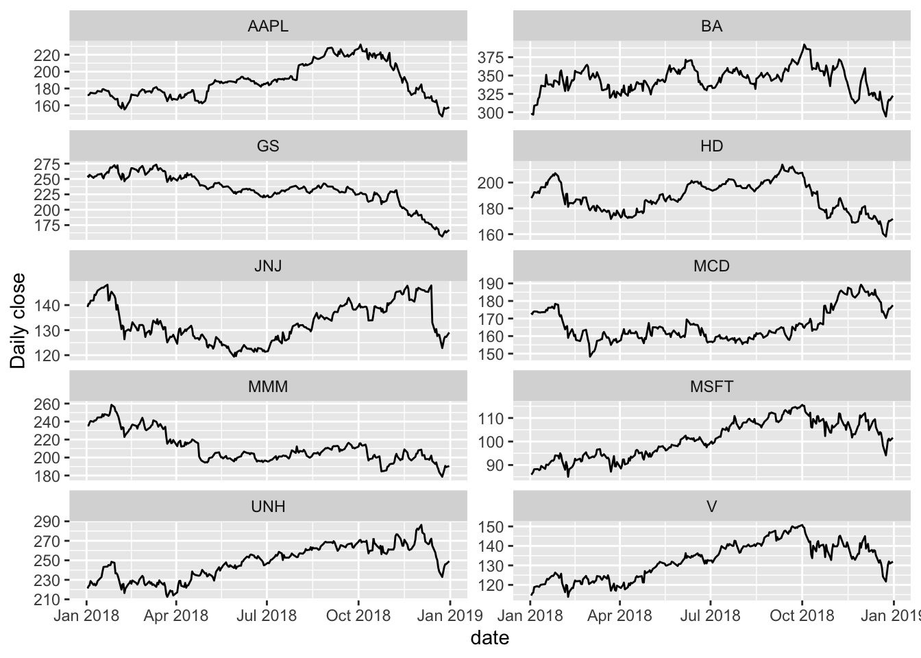

I want to explore the stock volatility, so I also look at the log daily returns rather than the closing price.

stockDF <- stockDF %>% dplyr::mutate(logR=log(close/dplyr::lag(close))) %>% dplyr::filter(date != date("2018-01-02"))
ggplot(stockDF, aes(x=date, y=logR))+
  geom_line()+
  facet_wrap(~symbol, scales='free_y', ncol=2)+
  xlim(c(date("2018-01-03"), date("2018-12-31")))+
  ylab("Daily log return")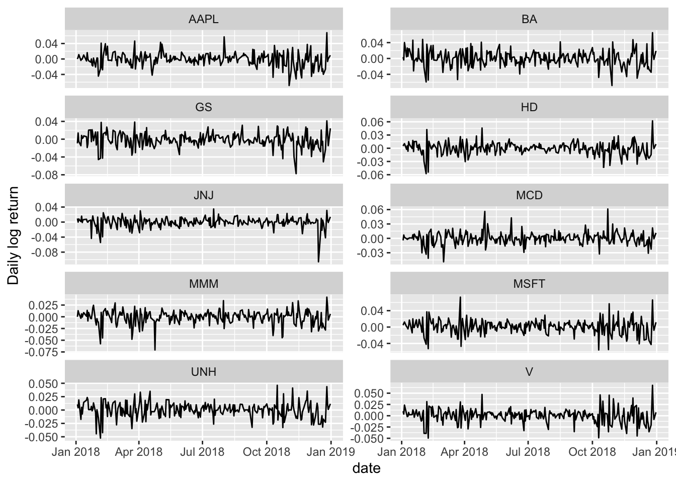

We see that the behavior of volatility tends to be similar across the different stocks. Particularly, there appears to be greater volatility during the beginning and end of this time period than during the middle. This could be useful when modeling this data, as we may be able to account for correlation between the stocks.