Nonlinear Small Area Estimation in R with nlfh

Installing nlfh

nlfh is available on CRAN and can be installed in the usual way.

install.packages("nlfh")

We will also use a few packages for data manipulation and mapping.

library(nlfh)
library(dplyr)
library(ggplot2)
library(sf)
library(tigris)
library(viridis)

The example data

The package includes acs_dat, an example data set with 1,617 Missouri census tracts. MedInc is the direct estimate of median household income and MedIncSE is its standard error. The remaining columns contain tract-level covariates.

data(acs_dat)
tract_geoid <- rownames(acs_dat)
acs_mo <- as.data.frame(acs_dat)
acs_mo$GEOID <- tract_geoid

head(acs_mo)

##   MedInc  MedIncSE  SNAPRate   PovRate     White       Black   Hispanic
## 1  75448 17981.763 0.4723866 0.1992110 0.5925325 0.300324675 0.03246753
## 2  33434  1093.009 0.3852814 0.3160173 0.2774533 0.538551402 0.09988318
## 3  57969  5765.957 0.6087978 0.1496904 0.4821522 0.360104987 0.05564304
## 4  60743  3502.128 0.3817734 0.1190476 0.9178744 0.003360639 0.01554295
## 5  58421  4869.909 0.3766943 0.1019624 0.8944666 0.014261266 0.02129682
## 6  43547  4725.228 0.4859327 0.2281346 0.7823583 0.068202486 0.05365262
##         Asian       GEOID
## 1 0.019480519 29510123200
## 2 0.008761682 29510124600
## 3 0.046456693 29510125500
## 4 0.004410838 29101960900
## 5 0.002662103 29101960200
## 6 0.015459230 29101960600

For a Fay–Herriot model, we supply the direct estimate and its known sampling variance. Because the data provide a standard error, the sampling variance is MedIncSE^2.

It is helpful to first look at the direct estimates on a map. The row names in acs_dat are census tract GEOIDs, so they can be joined directly to Census Bureau tract boundaries downloaded with tigris.

options(tigris_use_cache = TRUE)

mo_tracts <- tracts(
  state = "MO",
  year = 2020,
  cb = TRUE,
  class = "sf"
)

map_data <- mo_tracts |>
  left_join(acs_mo, by = "GEOID") |>
  filter(!is.na(MedInc))

ggplot(map_data) +
  geom_sf(aes(fill = MedInc), color = NA) +
  scale_fill_viridis_c(
    option = "mako",
    labels = scales::label_dollar(scale = 0.001, suffix = "k"),
    name = "Direct\nestimate"
  ) +
  labs(
    title = "Direct estimates of median household income",
    subtitle = "Missouri census tracts"
  ) +
  theme_void(base_size = 13) +
  theme(
    plot.title = element_text(face = "bold"),
    legend.position = "right"
  )

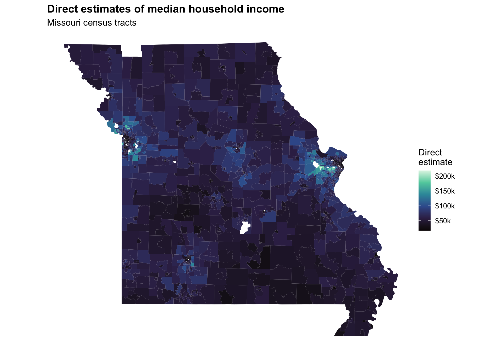
There is real geographic structure in the direct estimates, but the estimates are not equally precise. Some of the sharp differences between neighboring tracts may reflect signal, while others may reflect sampling variability. The purpose of the model is not to erase this variation. It is to account for the uncertainty when estimating the underlying tract-level values.

Fitting a nonlinear Fay–Herriot model

The main user-facing function in the package is fit_fh(). Its formula interface should look familiar to R users. For nonlinear models, the formula identifies which predictors are available to the model, but it does not restrict their effects to be linear or additive.

Here I use Bayesian additive regression trees (BART) for the mean function.

set.seed(2026)

fit_bart <- fit_fh(
  MedInc ~ SNAPRate + PovRate + White + Black + Hispanic + Asian,
  sampling_variance = MedIncSE^2,
  data = acs_mo,
  method = "bart",
  control = list(
    n_iter = 1000,
    burn_in = 500,
    progress = FALSE
  )
)

summary(fit_bart)

## <summary.nlfh_fit>
## Model type: BART Fay-Herriot
## Formula: MedInc ~ SNAPRate + PovRate + White + Black + Hispanic + Asian
## DIC: 36957
## 
## MCMC:
##  n_iter burn_in posterior_draws areas
##    1000     500             500  1617
## 
## Details:
##  retained_draws burn_in_fraction progress scale n_trees n_bart_samples
##             500              0.5    FALSE FALSE      50             10
## 
## Variance parameters:
##               parameter   mean     sd median   q2.5  q97.5
##  random_effect_variance 0.3345 0.1418 0.3158 0.1269 0.6531
## 
## Area-level estimates theta_i:
##  area  mean   sd median  q2.5 q97.5
##     1 47520 3161  47730 41590 53530
##     2 34750 1406  34880 31640 37120
##     3 44190 2906  43840 39480 50350
##     4 54080 1401  53690 52180 57450
##     5 61940 1602  61830 59260 65130
##     6 31260 3048  30730 26190 37860
## ... 1611 more rows
## 
## Variable importance:
##   SNAPRate    PovRate      White      Black   Hispanic      Asian 
## 0.17216191 0.24776581 0.17140518 0.16129210 0.09538537 0.15198963

The model estimates an unspecified nonlinear function of the six predictors and adds a tract-level random effect. At the same time, it retains the Fay–Herriot sampling model, so direct estimates with large standard errors are allowed to borrow more information than highly precise direct estimates.

The fitted model contains full posterior draws, not just point estimates. For a quick summary, fitted() returns the posterior mean for each tract. Setting full = TRUE also returns posterior standard deviations and credible intervals.

tract_estimates <- fitted(fit_bart, full = TRUE)

map_data <- map_data |>
  mutate(
    model_estimate = tract_estimates$mean[
      match(GEOID, acs_mo$GEOID)
    ],
    model_sd = tract_estimates$sd[
      match(GEOID, acs_mo$GEOID)
    ]
  )

head(tract_estimates)

##   area     mean       sd   median     q2.5    q97.5
## 1    1 47516.53 3160.589 47733.40 41591.80 53530.76
## 2    2 34754.31 1406.342 34881.56 31637.93 37119.98
## 3    3 44193.09 2905.727 43842.86 39478.27 50346.72
## 4    4 54084.83 1400.874 53689.90 52184.31 57447.70
## 5    5 61942.29 1602.468 61833.78 59259.85 65131.50
## 6    6 31256.79 3047.542 30725.50 26186.71 37859.11

What changed?

The most useful comparison is between the noisy direct estimates and the posterior estimates of the underlying tract means.

comparison_map <- map_data |>
  transmute(
    GEOID,
    Estimate = "Direct",
    Income = MedInc
  )

comparison_map <- bind_rows(
  comparison_map,
  map_data |>
    transmute(
      GEOID,
      Estimate = "BART-FH",
      Income = model_estimate
    )
)
comparison_map$Estimate <- factor(
  comparison_map$Estimate,
  levels = c("Direct", "BART-FH")
)

ggplot(comparison_map) +
  geom_sf(aes(fill = Income), color = NA) +
  facet_wrap(~Estimate, ncol = 2) +
  scale_fill_viridis_c(
    option = "mako",
    limits = range(comparison_map$Income, na.rm = TRUE),
    labels = scales::label_dollar(scale = 0.001, suffix = "k"),
    name = "Median\nincome"
  ) +
  labs(
    title = "From direct estimates to small area estimates",
    subtitle = "The same color scale is used in both maps"
  ) +
  theme_void(base_size = 13) +
  theme(
    plot.title = element_text(face = "bold"),
    strip.text = element_text(face = "bold", size = 12),
    legend.position = "right"
  )

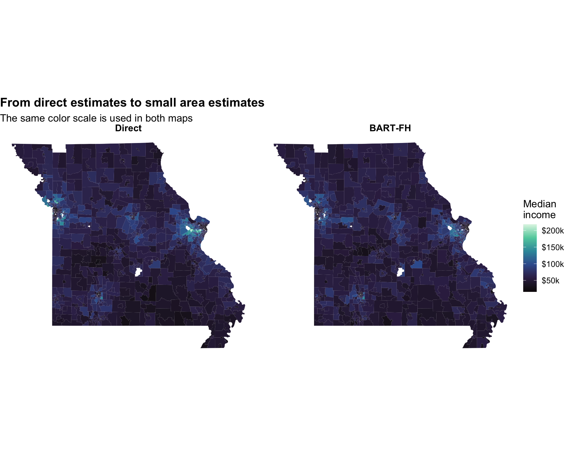
The broad spatial pattern remains, but some of the most extreme local values move toward estimates supported by the covariates and the rest of the data. This is the usual small area estimation tradeoff: we accept a model in order to reduce the instability of direct estimates.

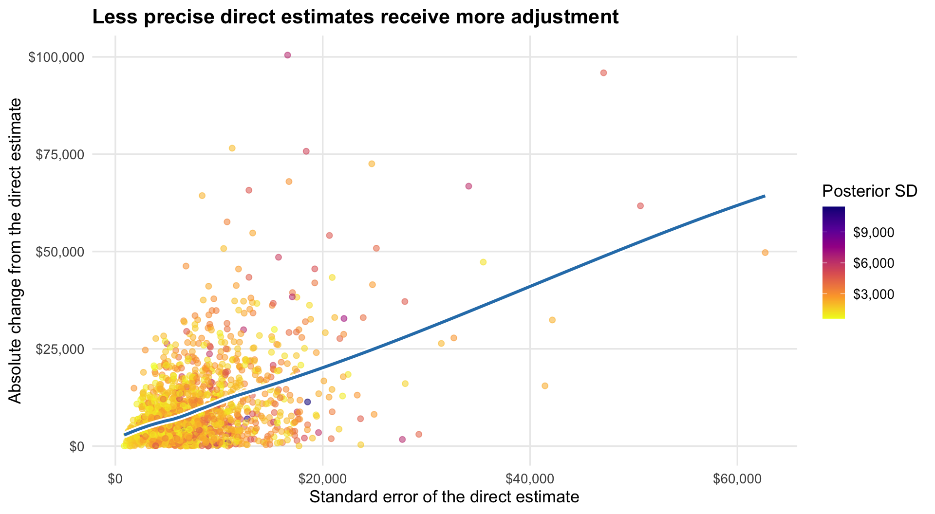
The amount of movement is not constant. Tracts with larger direct-estimate standard errors generally have more to gain from the model.

ggplot(
  map_data,
  aes(x = MedIncSE, y = abs(model_estimate - MedInc))
) +
  geom_point(
    aes(color = model_sd),
    alpha = 0.55,
    size = 1.8
  ) +
  geom_smooth(method = "loess", color = "white", linewidth = 2.4, se = FALSE) +
  geom_smooth(method = "loess", color = "#2c7fb8", linewidth = 1.1, se = FALSE) +
  scale_color_viridis_c(
    option = "plasma",
    direction = -1,
    name = "Posterior SD",
    labels = scales::label_dollar()
  ) +
  scale_x_continuous(labels = scales::label_dollar()) +
  scale_y_continuous(labels = scales::label_dollar()) +
  labs(
    title = "Less precise direct estimates receive more adjustment",
    x = "Standard error of the direct estimate",
    y = "Absolute change from the direct estimate"
  ) +
  theme_minimal(base_size = 13) +
  theme(
    plot.title = element_text(face = "bold"),
    panel.grid.minor = element_blank()
  )

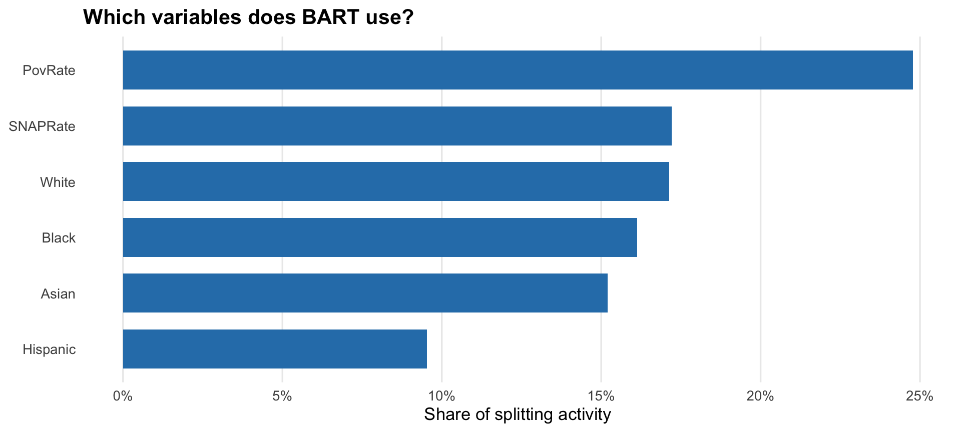
For the BART model, variable_importance gives the proportion of splitting activity attributed to each predictor. This is a useful model diagnostic, although it should not be interpreted as a causal effect.

importance <- data.frame(
  variable = names(fit_bart$variable_importance),
  importance = as.numeric(fit_bart$variable_importance)
) |>
  arrange(importance) |>
  mutate(variable = factor(variable, levels = variable))

ggplot(importance, aes(x = importance, y = variable)) +
  geom_col(fill = "#2c7fb8", width = 0.7) +
  scale_x_continuous(labels = scales::label_percent()) +
  labs(
    title = "Which variables does BART use?",
    x = "Share of splitting activity",
    y = NULL
  ) +
  theme_minimal(base_size = 13) +
  theme(
    plot.title = element_text(face = "bold"),
    panel.grid.major.y = element_blank(),
    panel.grid.minor = element_blank()
  )

One interface, three models

BART is only one option. Changing the method argument fits the standard linear Fay–Herriot model or the random-weight neural network model using the same general interface.

fit_linear <- fit_fh(
  MedInc ~ SNAPRate + PovRate + White + Black + Hispanic + Asian,
  sampling_variance = MedIncSE^2,
  data = acs_mo,
  method = "linear"
)

fit_rnn <- fit_fh(
  MedInc ~ SNAPRate + PovRate + White + Black + Hispanic + Asian,
  sampling_variance = MedIncSE^2,
  data = acs_mo,
  method = "rnn"
)

All three methods return objects with a common set of tools. summary() reports posterior summaries, fitted() extracts area-level estimates, and posterior_draws() makes the retained simulations available for custom summaries or uncertainty propagation. The model objects also contain DIC for comparisons among models fit to the same data. As always, I would use model comparison together with diagnostics and substantive knowledge, rather than treating a single criterion as the final answer.

Why use nlfh?

The goal of nlfh is to make nonlinear small area estimation feel like a normal R workflow. A user can start with a formula, a vector of sampling variances, and one call to fit_fh(). The package handles the model fitting while still returning the posterior quantities needed for a serious analysis.

More importantly, it provides an alternative to two common estimation choices. We do not have to rely on unstable direct estimates, and we do not have to assume that the relationship between an outcome and its predictors is linear. BART and the random-weight neural network allow the data to support nonlinearities and interactions while retaining the familiar area-level sampling model.

You can find the package on CRAN and the source code on GitHub.